How to Create a Dropdown List in Excel that Actually Works

If you’ve ever struggled to keep data entry clean and consistent in your Excel worksheets, you’re not alone. One of the most common problems in Excel is messy data: people type things differently, misspell words, or simply forget what’s allowed. That’s where dropdown lists in Excel come to the rescue.

In this guide, I’ll show you how to create dropdown lists in Excel using data validation, explore different methods (from simple to advanced), and share troubleshooting tips I’ve learned over years of training everyday Excel users. By the end, you’ll not only know how to build dropdowns but also how to make them dynamic, flexible, and foolproof.

Why Use Dropdown Lists in Excel?

Dropdowns, more formally known as Excel’s Data Validation Lists, are useful when you need to:

• Improve accuracy and consistency - A dropdown list prevents typos and inconsistent entries like “CA” vs. “Calif.” vs. “California.” Everyone picks from the same standardized set of choices.
• Save time on data entry - Instead of typing everything, users can simply click and choose from the menu.
• Make your spreadsheets more professional - Dropdowns give your workbooks a polished, user-friendly feel that makes it easier for others to interact with your spreadsheets.

It is best to avoid dropdowns when:

• Users must routinely select many values at once - Excel has no native multi-select from a list.
• Your list is huge (thousands of items) and users need to search to locate their specific choice. There is no ability to search inside a dropdown list.

How to Create a Dropdown List in Excel (Step-by-Step)

There are several ways to create dropdown lists in Excel. Let’s look at them from simplest to most advanced.

Method 1: Simple list typed directly into data validation

This method is best for short, static choices in your list. It’s a fast, no setup method, but the downsides are that this method is limited in what it can do and is hard to maintain. This list is typed in a comma-delimited string and is character-limited to 255.

These lists cannot grow dynamically. If you need to update the list, you must repeat the steps below and update the list string. If your list is unlikely to change, this might be the right type for you. Here’s how we create them:

1. Select the cell (or range of cells) where you want the dropdown.
2. Go to the Data tab on the Ribbon.
3. Click Data Validation (in the Data Tools group).
4. In the Allow box, choose List.
5. In the Source box, type your items separated by commas, for example: Yes,No,Maybe
6. Click OK.

Method 2: Dropdown list from a cell range

This method is the best to use if the data list may be updated at any point. Here, we will show Excel a range in our spreadsheet that contains the list. Whatever content is in the range will be the available data choices for the list.

Updating the content in the future will automatically update the list without the need to return to the Data Validation dialog box. However, adding items beyond the selected range won’t appear unless you extend the source in the data validation dialog box.

1. Type your list of items in a column (e.g., A2:A10).
2. Select the cell(s) for your dropdown.
3. Go to the Data tab on the Ribbon.
4. Click Data Validation (in the Data Tools group).
5. In the Allow box, choose List.
6. In the Source box, highlight your range (e.g., =$A$2:$A$10).
7. Pro Tip: If you have more than one valid list in your spreadsheet, it can be beneficial to name your ranges using the Name Manager feature on the Formulas tab on the Ribbon. 
8. Click OK.

Method 3: Use an Excel Table for automatic expansion

This method is great if you suspect a need for additional items in the dropdown in the future. By formatting your list as an Excel Table, you can add items to the table and the dropdown list will automatically be updated since the link is to the defined table and not a cell range. 

To use this method, you will be creating a formula in the Source box. The specific formula we will use is =INDIRECT. If you are unfamiliar with this formula, =INDIRECT is a tool that lets you point to a cell, or in our case table range, without locking it in.

Instead of typing a cell address directly into your formula, you can use =INDIRECT to create one that changes based on your needs. The big advantage is that you don’t have to rewrite the whole formula if you want it to look somewhere else. Plus, these references won’t break or shift around if you add or delete rows or columns in your sheet, which is exactly what we need.

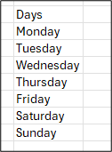
• 1. Enter your list in a column. While a column header is not necessary, it is helpful. Below, “Days” is the column header and the list follows.

• Select the list and press Ctrl + T (or go to the Insert tab and select Table).
• Check My table has headers if you have added one as suggested.
• Move to the area in your workbook where you want to input the data and select the desired input cell(s).
• Go to the Data tab on the Ribbon.
• Click Data Validation (in the Data Tools group).
• In the Allow box, choose List.
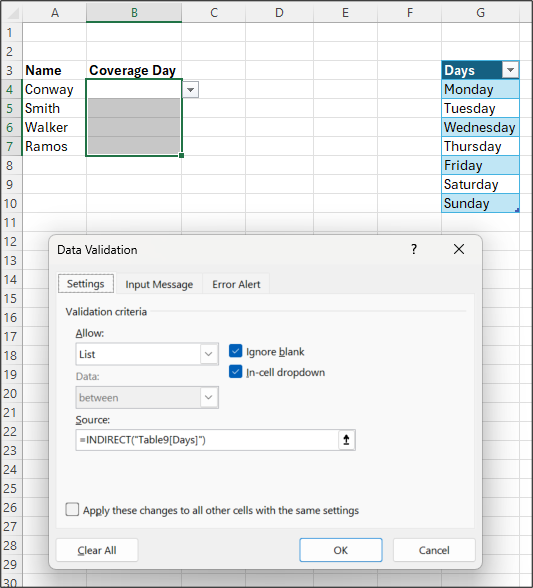
• In the Source box, enter your formula: =INDIRECT(“Table_name[Column_name]”)
• Click OK to finish.

In the example below, the dropdown menu is created from the “Days” column in Table1. The formula looks like this: =INDIRECT(Table1[Days]”)

Method 4: Dynamic dropdown lists with formulas (spilled ranges)

If you’re using Microsoft 365 or Excel 2021+, you can take advantage of dynamic arrays. This method is similar to Method 3 above but is beneficial if the table from which you are drawing your dropdown list has repeated values. In Method 3, every duplicate will appear in the dropdown validation list creating bloat and confusion. With spilled ranges, we can have Excel create an extracted list of unique entries from which to create the dropdown list. 

For example, let’s say you have a list of departments in your worksheet:

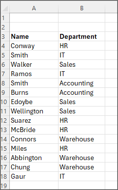
And you want to pull the departments from Column B to use for inputting data in another table, like Column H in the example below. This is where a spilled range will come in handy.

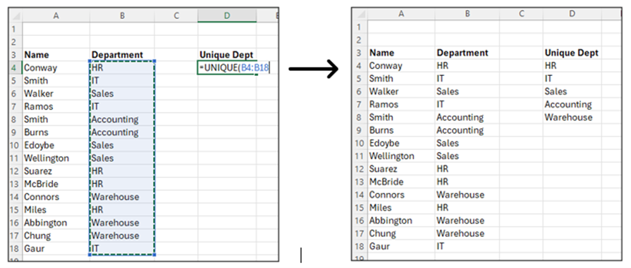
The first step is to extract the unique list from the data in Column B.

• In an empty cell in your workbook, enter the formula: =UNIQUE(range). Here the range is the source data currently lives. In our example above, the formula would be =UNIQUE(B4:B18).

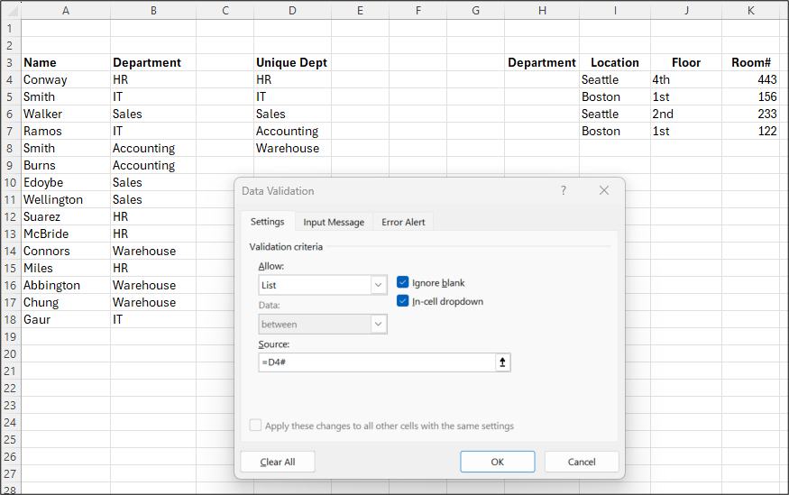
• Next, select the cells where you want your dropdown list to appear.
• Go to the Data tab on the Ribbon.
• Click Data Validation (in the Data Tools group).
• In the Allow box, choose List.
• In the Source box, you merely need to add the cell address of the first cell in the list followed by #. The # tells Excel to use the entire spilled range from our =UNIQUE formula. This allows the length of the list to expand or contract based on changes from the source without the need to reset the validation list! In our example, the formula will be: =D4#

If “Marketing” is added to the source list in Column B, “Marketing” will automatically appear in the Unique list in Column D and be available from the drop down validation.

Method 5: Create dependent (cascading) dropdown lists

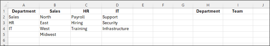
Sometimes you need one dropdown to depend on another. For example, you have a list of departments, but each department also has specific teams within it:

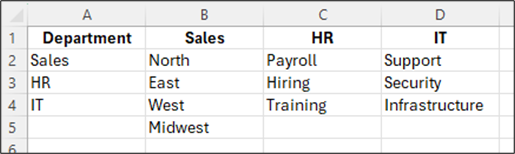
• Dropdown 1: Department (Sales, HR, IT).
• Dropdown 2: The specific teams available based on the department selected.

First, we need to create named ranges for each team:

• Select the first team. In our example above, that would be B2:B5.
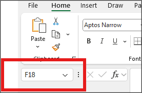
• Click in the Range Name box (highlighted in the image below) and type Sales. Press Enter to confirm the range name. 

• Repeat for HR and IT selecting the specific range for each and naming them HR and IT respectively. 

Now we’re ready to create the validation lists. 

• First create the data entry locations. In our example below, our department validation list will appear in Column H and the corresponding Team validation list will appear in Column I.

• Select the range cells in column H in which you want the Department validation list to appear.
• Go to the Data tab on the Ribbon.
• Click Data Validation (in the Data Tools group).
• In the Allow box, choose List.
• In the Source box, type the range in which the department list can be found. In our example it would be =A2:A4.
• Click OK to complete the first validation list.
• Next, select the range cells in column I in which you want the Teams validation list to appear.
• Go to the Data tab on the Ribbon.
• Click Data Validation (in the Data Tools group).
• In the Allow box, choose List.
• In the Source box, type =INDIRECT(H2). The H2 reference will let Excel see the department selected. The INDIRECT function will have Excel look for a range with the same name and extract the data from that range to create the list.
• Click OK to complete the second validation list.

Customizing Dropdown Lists

PHEW! Now that we know all the various ways to create validation lists, let’s quickly review a couple of final things we can customize any time we create these lists.

Input Message

The first option is to offer users guidance on using the dropdown lists. 

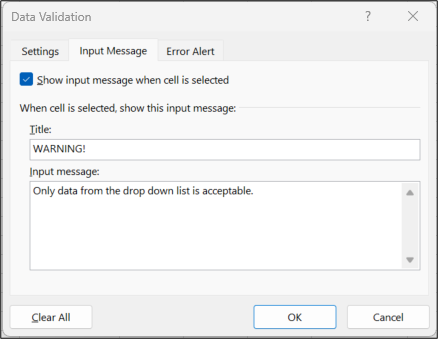
1. In the Data Validation dialog box, click the Input Message tab.
2. Enter text in the Title field to display in the title bar of an input message.
3. Enter guidance like “Only data from the drop down list is acceptable” in the Input message field. 
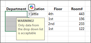
4. Click OK. When a user clicks into a cell using the validation list, a yellow message explaining the use will appear:

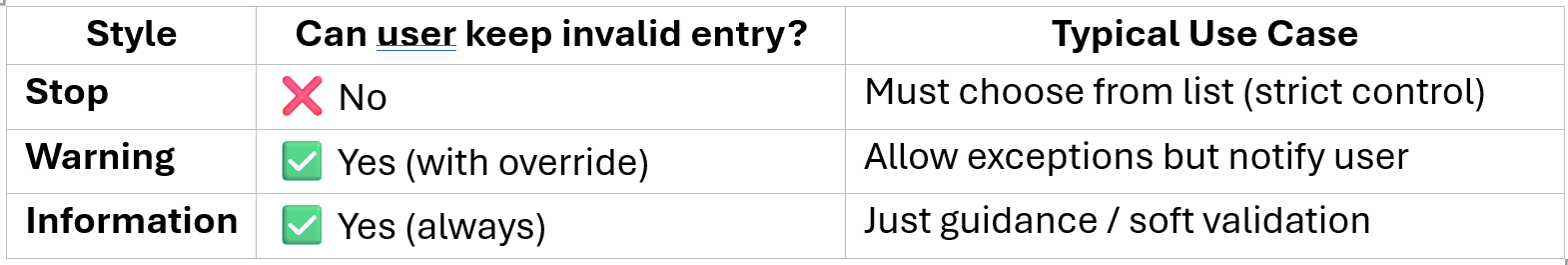
Error Alert

The Error Alert option allows you to let users know when they have entered invalid data. There are three types of Error Alerts:

• In the Data Validation dialog box, click the Error Alert tab.
• From the Style list, select Stop, Warning, or Information.
• As with creating an Input Message, enter a title and the error message you want displayed when the user enters incorrect data. Example:

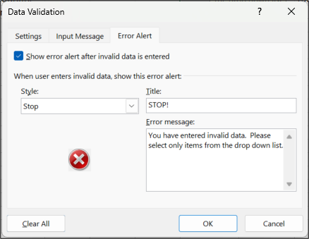
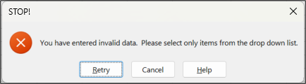
• Click OK to finish. Below is what the error alert will look like:

Common Problems with Excel Dropdown Lists (and Fixes)

• Dropdown arrow not showing - Check whether the worksheet is protected or the cell is hidden.
• Blank cells appearing in the list - Use the FILTER function or clean your source range to remove empty rows.
• Character limits when typing items directly - The comma-separated list method has a 255-character limit. Use a range instead.
• Dependent lists not working properly - Ensure your named ranges match exactly. Remember, Excel doesn’t allow spaces in range names.

Real-World Examples of Dropdown Lists in Excel

• HR and employee data - Select job titles, departments, or locations consistently.
• Finance and expense categories - Ensure expense tracking uses standard categories.
• Sales and product tracking - Pick product names or customer types without spelling errors.
• Project management and task status - Standardize status updates with “Not Started, In Progress, Completed.”

Advanced Tips from an Excel Trainer

• Combine dropdowns with conditional formatting - Make selections more visual by coloring them automatically.
• Use named ranges for easier management - Instead of cell references, name your ranges (e.g., Departments).
• Hide your source list to keep sheets clean - Place your source data on a separate, hidden sheet.
• Sort and filter dropdowns with dynamic arrays - Use formulas like: SORT(UNIQUE(FILTER(A2:A100,A2:A100<>"")))
• This ensures your dropdown is both alphabetical and duplicate-free.

Key Takeaways

• Dropdown lists in Excel are created using Data Validation.
• You can build them from typed lists, ranges, Tables, or formulas.
• Dropdowns improve accuracy, speed, and consistency in spreadsheets.
• Advanced options include dependent dropdowns and dynamic spilled lists.
• Common pitfalls include blanks, character limits, and validation errors.

Final Thoughts

If you’ve never used dropdown lists before, start with the simple comma-separated method. Once you’re comfortable, try range-based lists, Tables, and dynamic arrays. With just a little practice, you’ll create dropdowns that not only make your Excel sheets cleaner and easier to use but also impress your colleagues.

Remember: Excel is most powerful when it keeps your data accurate. Dropdown lists are one of the simplest yet most effective ways to make that happen.

Take Your Excel Skills Even Further

Mastering dropdown lists is just the beginning of what Excel can do for you. If you’re ready to unlock more powerful features, Intellezy’s comprehensive library of professional training courses has you covered. With thousands of short, searchable lessons, you can learn at your own pace and immediately apply new skills on the job.

Whether you’re just getting started or looking to advance your expertise, our online Excel courses are designed for every level:

• Excel Training for Beginners – Build a strong foundation with essential skills, formulas, and formatting.
• Excel Intermediate Training – Take your knowledge further with PivotTables, charts, and data tools.
• Advanced Excel 365 Course – Harness the power of dynamic arrays, advanced formulas, and automation.
• Excel Expert Training – Master complex data analysis, modeling, and advanced productivity features.
• And more!

Explore our Excel courses and start your free trial today.

Frequently Asked Questions about Dropdown Lists in Excel

1. How do I create a dropdown list in Excel?

Go to Data → Data Validation → List, then either type items separated by commas (e.g., Yes,No,Maybe) or select a range of cells containing your list.

2. Can I create a dropdown list that updates automatically?

Yes. The easiest way is to store your list in an Excel Table. When you add new items to the Table, the dropdown expands automatically. For more advanced users, you can also use dynamic array formulas like =UNIQUE(FILTER(A2:A100,A2:A100<>"")).

3. What is the maximum number of items in an Excel dropdown list?

If you type items directly into the Source box, there’s a 255-character limit (including commas). To avoid this limit, store your list in a cell range or Table instead.

4. Can I make a dropdown list depend on another dropdown?

Yes. This is called a dependent or cascading dropdown list. It typically requires naming ranges for each main category and using the INDIRECT function so the second dropdown updates based on the first.

5. Why isn’t my dropdown arrow showing in Excel?

Common reasons include:

• The worksheet is protected.
• The cell is too small to display the arrow.
• Data validation was not applied correctly.

Check these settings and reapply validation if needed.